Probability of Failure Module
The Lifetime Probability of Failure Model is used to conduct lifetime probability of failure analysis. It is capable of producing the probabilistic prediction curves (decay curves) based on pipe failure mechanism and statistical information of key physical parameters.
To discuss your results, please send your results to our experts at Monash University. If you are having difficulties with the platform, please see the help files associated with each of the of the components or please email us at civeng-crcp-l@monash.edu with your data files.
Lifetime Probability of Failure
Pipe Properties
Failure History
Time period for the recorded number of failures (years):
The period of time during which the number of past failures were recorded. The time period for the recorded number of failures should be non-negative.
Accepted Values: 0 ≤ years
(Click to see User Manual - Pipe failure analysis for more information)
Accepted Values: 0 ≤ years
(Click to see User Manual - Pipe failure analysis for more information)
Number of past failures:
The number of failures which has been recorded in the past. The number of past failures should be non-negative.
Accepted Values: 0 ≤ no. of past failures
(Click to see User Manual - Pipe failure analysis for more information)
Accepted Values: 0 ≤ no. of past failures
(Click to see User Manual - Pipe failure analysis for more information)
Soil Properties
Soil modulus (MPa):
An elastic soil parameter used in the settlement, compression or movement of soils. It is the slope of stress–strain curve in the elastic deformation region for the soil.
Accepted Values: 0 < Es
(Click to see User Manual - Pipe failure analysis for more information)
Accepted Values: 0 < Es
(Click to see User Manual - Pipe failure analysis for more information)
Lateral earth pressure coefficient:
The lateral earth pressure coefficient at rest and can be calculated by: k = ( 1 - sin∅ ) where ∅ is the soil friction angle.
Accepted Values: 0 ≤ 1
(Click to see User Manual - Pipe failure analysis for more information)
Accepted Values: 0 ≤ 1
(Click to see User Manual - Pipe failure analysis for more information)
Soil unit weight (kN/m3):
The ratio of the total weight of soil to the total volume of soil. Soil unit weight or bulk unit weight is the unit weight of soil and varies for different soil types. The values are typically between 15 kN/m3 to 20 kN/m3.
Accepted Values: 0 < γs ≤ 30 kN/m3
(Click to see User Manual - Pipe failure analysis for more information)
Accepted Values: 0 < γs ≤ 30 kN/m3
(Click to see User Manual - Pipe failure analysis for more information)
Loading
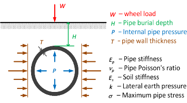
Traffic load (kN):
Indicated by the wheel load. Click to see the image A buried pipe under internal pressure and traffic load for more information.
Accepted Values: 0 ≤ W < 100 kN
(Click to see User Manual - Pipe failure analysis for more information)
Accepted Values: 0 ≤ W < 100 kN
(Click to see User Manual - Pipe failure analysis for more information)
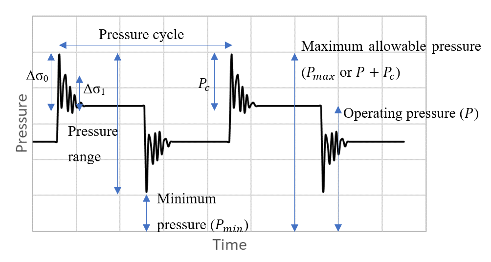
Maximum allowable pressure (kPa):
The maximum pressure in the pipe taking into account surge pressure. Click to see the image Pressure explanations for more information.
Accepted Values: 0 ≤ Pmax
(Click to see User Manual - Pipe failure analysis for more information)
Accepted Values: 0 ≤ Pmax
(Click to see User Manual - Pipe failure analysis for more information)
Corrosion Model
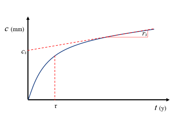
Long-term, steady state corrosion rate of metallic pipes:
Click to see the image Power law model used for corrosion level estimation for more information.
Accepted Values: 0 ≤ rs ≤ 1
(Click to see User Manual - Pipe failure analysis for more information)
Accepted Values: 0 ≤ rs ≤ 1
(Click to see User Manual - Pipe failure analysis for more information)
Intercept parameter for long-term corrosion of metallic pipes:
Click to see the image Power law model used for corrosion level estimation for more information.
Accepted Values: 0 ≤ cs ≤ 50
(Click to see User Manual - Pipe failure analysis for more information)
Accepted Values: 0 ≤ cs ≤ 50
(Click to see User Manual - Pipe failure analysis for more information)
Transition period between short-term and long-term corrosion:
The time it takes for the pit depth to attain around 63% of the maximum value in the absence of long-term corrosion rates (i.e., rs = 0). If no value is available, then a value of 15 years is suggested to be used according to a careful review of the existing data in literature. Click to see the image Power law model used for corrosion level estimation for more information.
Accepted Values: 0 ≤ τ ≤ 100 years
(Click to see User Manual - Pipe failure analysis for more information)
Accepted Values: 0 ≤ τ ≤ 100 years
(Click to see User Manual - Pipe failure analysis for more information)
Aspect ratio:
Calculated by dividing half of the corrosion patch length (a) by patch depth (c). This ratio determines how the corrosion patch grows in the longitudinal and radial directions. A proper value can be selected based on the inspection of the corrosion patches identified from the scanned thickness maps of the excavated pipe segments.
k2 = a ÷ c
Accepted Values: 0 ≤ k2 ≤ 100
(Click to see User Manual - Pipe failure analysis for more information)
k2 = a ÷ c
Accepted Values: 0 ≤ k2 ≤ 100
(Click to see User Manual - Pipe failure analysis for more information)
Patch factor:
calculated by dividing the corrosion patch length (2a) by patch width (2b). This ratio determines how the corrosion patch grows in the longitudinal and circumferential directions. A proper value can be selected based on the inspection of the corrosion patches identified from the scanned thickness maps of the excavated pipe segments.
k1 = 2a ÷ 2b
Accepted Values: 0 ≤ k1 ≤ 1000
(Click to see User Manual - Pipe failure analysis for more information)
k1 = 2a ÷ 2b
Accepted Values: 0 ≤ k1 ≤ 1000
(Click to see User Manual - Pipe failure analysis for more information)